Lorem ipsum dolor sit amet, consectetur adipiscing elit, sed do eiusmod tempor incididunt ut labore et dolore magna aliqua. Ut enim ad minim veniam, quis nostrud exercitation ullamco laboris nisi ut aliquip ex ea commodo consequat. Duis aute irure dolor in reprehenderit in voluptate velit esse cillum dolore eu fugiat nulla pariatur. Excepteur sint occaecat cupidatat non proident, sunt in culpa qui officia deserunt mollit anim id est laborum.

TextStar

A lightweight Julia package for simulating the dynamics of a configuration of trapped ions interacting with laser light. 

IonSim leverages QuantumOptics.jl to deliver a performant, quantitatively faithful tool for simulating fundamental interactions in trapped ion experiments. Several ion species and trap configurations are implemented and everything is written in the language of experimentalists (ions and lasers, not qubits and gates).

Code Examples


using IonSim
using QuantumOptics

# Construct the system
C = Ca40([("S1/2", -1/2), ("D5/2", -1/2)])
set_sublevel_alias!(C, Dict("S" => ("S1/2", -1/2),
                            "D" => ("D5/2", -1/2)))
L1 = Laser(ϕ=π); L2 = Laser()  # note the π-phase between L1/L2
chain = LinearChain(ions=[C, C], com_frequencies=(x=3e6, y=3e6, z=2.5e5),
        vibrational_modes=(;z=[1]))
T = Trap(configuration=chain, B=6e-4, Bhat=(x̂ + ẑ)/√2,
        lasers=[L1, L2])
mode = T.configuration.vibrational_modes.z[1]

# Set the laser parameters
ϵ = 10e3
d = 350  # correct for single-photon coupling to sidebands
L1.λ = transitionwavelength(C, ("S", "D"), T)
L2.λ = transitionwavelength(C, ("S", "D"), T)
L1.Δ = mode.ν + ϵ - d
L2.Δ = -mode.ν - ϵ + d
L1.k = L2.k = ẑ
L1.ϵ = L2.ϵ = x̂
# set 'resonance' condition: ηΩ = 1/2ϵ
η = abs(get_η(mode, L1, C))
E = Efield_from_pi_time!(η/ϵ, T, 1, 1, ("S", "D"))(0)
Ω = t -> t < 20 ? E * sin(2π * t / 80)^2 : E  # ampl. ramp
L1.E = L2.E = Ω

# Build Hamiltonian
h = hamiltonian(T, lamb_dicke_order=1, rwa_cutoff=Inf)

# Solve
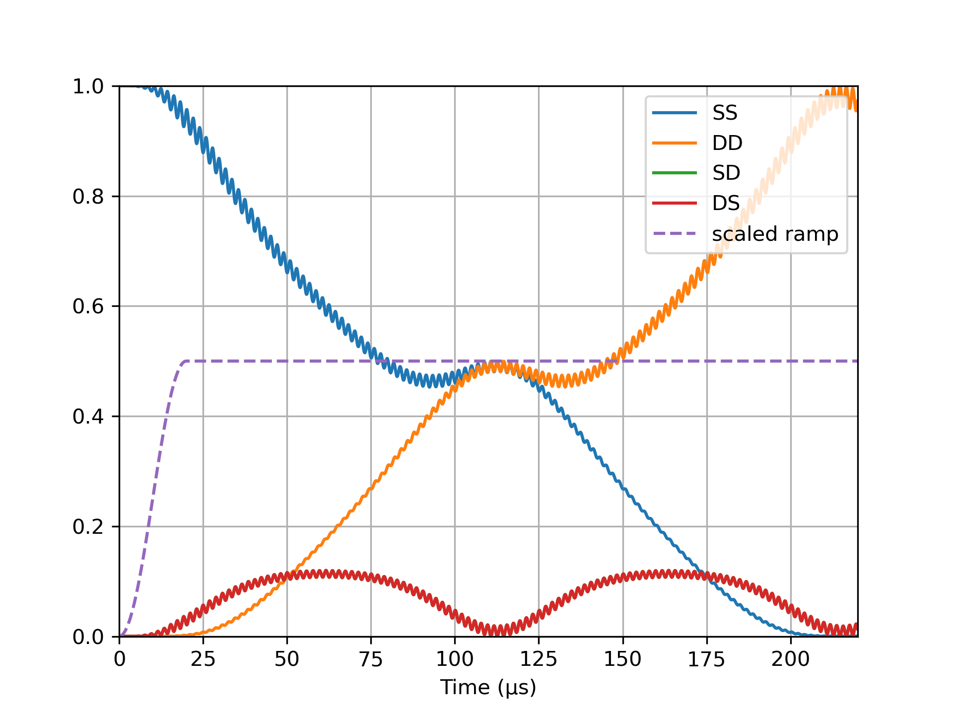
t, sol = timeevolution.schroedinger_dynamic(0:.1:220, C["S"] ⊗ C["S"] ⊗ mode[0], h);

import PyPlot
const plt = PyPlot

SS = expect(ionprojector(T, "S", "S"), sol)
DD = expect(ionprojector(T, "D", "D"), sol)
SD = expect(ionprojector(T, "S", "D"), sol)
DS = expect(ionprojector(T, "D", "S"), sol)
plt.plot(t, SS, label="SS")
plt.plot(t, DD, label="DD")
plt.plot(t, SD, label="SD")
plt.plot(t, DS, label="DS")
plt.plot(t, @.(Ω(t) / 2E), ls="--", label="scaled ramp")
plt.legend(loc=1)
plt.xlim(t[1], t[end])
plt.ylim(0, 1)
plt.xlabel("Time (μs)")
plt.grid()

using IonSim
using QuantumOptics

# Construct the system
C = Ca40([("S1/2", -1/2), ("D5/2", -1/2)])
set_sublevel_alias!(C, Dict("S" => ("S1/2", -1/2),
                            "D" => ("D5/2", -1/2)))
L = Laser()
chain = LinearChain(
        ions=[C], com_frequencies=(x=3e6, y=3e6, z=1e6),
        vibrational_modes=(;z=[1])
    )
T = Trap(configuration=chain, B=4e-4, Bhat=ẑ, lasers=[L])

# Set the laser parameters
L.k = (x̂ + ẑ)/√2
L.ϵ = (x̂ - ẑ)/√2
L.λ = transitionwavelength(C, ("S", "D"), T)
Efield_from_pi_time!(2e-6, T, 1, 1, ("S", "D"))

# Set the vibrational mode Hilbert space dimension
mode = T.configuration.vibrational_modes.z[1]
mode.N = 100

# Construct initial state
ρi_ion = dm(C["S"])
ρi_mode = thermalstate(mode, 10)  # thermal state n̄=10
ρi = ρi_ion ⊗ ρi_mode

# Construct the hamiltonian
h = hamiltonian(T, timescale=1e-6)

# Solve the system
tout, sol = timeevolution.schroedinger_dynamic(0:.1:50, ρi, h);

import PyPlot
const plt = PyPlot

plt.plot(
        tout, expect(ionprojector(T, "D"), sol),
        label="Excited State Population"
    )
plt.xlim(tout[1], tout[end])
plt.ylim(0, 1)
plt.grid()
plt.xlabel("Time (μs)")
plt.legend(loc=1)

using IonSim
using QuantumOptics

# Construct the system
C = Ca40([("S1/2", -1/2), ("D5/2", -1/2)])
set_sublevel_alias!(C, Dict("S" => ("S1/2", -1/2),
                            "D" => ("D5/2", -1/2)))
L = Laser()
chain = LinearChain(
        ions=[C], com_frequencies=(x=3e6, y=3e6, z=1e6),
        vibrational_modes=(;z=[1])
    )
T = Trap(configuration=chain, B=2.9e-4, Bhat=ẑ, lasers=[L])

# Set the laser parameters
L.k = (x̂ + ẑ)/√2
L.ϵ = (x̂ - ẑ)/√2
L.λ = transitionwavelength(C, ("S", "D"), T)
# Set pi_time to 4 μs
E = Efield_from_pi_time(4e-6, T, 1, 1, ("S", "D"))

# We'll linearly sweep through the laser's frequency over
# [-125, +125] kHz (detuned from the carrier transition) in a time Tp
Tp = 250
Δϕ = Tp * 1e-3
L.ϕ = t -> 2π * (-Δϕ/2 + (Δϕ / Tp) * t) * t

# And also smoothly turn on and off the laser's electric field strength
Ω = t -> E * sin(π * t/Tp)^2
L.E = Ω

# Build Hamiltonian
h = hamiltonian(T, rwa_cutoff=Inf, lamb_dicke_order=1)

# Solve system
mode = T.configuration.vibrational_modes.z[1]
tout, sol = timeevolution.schroedinger_dynamic(0:.1:Tp, C["S"] ⊗ mode[0], h);

import PyPlot
const plt = PyPlot

plt.plot(tout, expect(ionprojector(T, "D"), sol),
        lw=3, color="C3", label="excited state population")
plt.plot(tout, @.(L.E(tout) / 2E),
        ls="--", label="scaled amplitude profile")
plt.plot(tout, @.(L.ϕ(tout) / (2π * Δϕ * tout)),
        ls="--", label="scaled frequency profile")
plt.xlim(tout[1], tout[end])
plt.legend(loc=4)
plt.grid()
plt.xlabel("Time (μs)")
  • Fast: runtimes comparable to QuTiP (Cython)
  • Intuitive: you set up your simulation the same way that you set up your experiments
  • Flexible: full control over RWA cutoff frequencies, Lamb-Dicke order approximations, Hilbert space truncation and methods
  • Open Source: all source code is freely available and built with extensibility in mind

IonSim is maintained by Hartmut Haeffner's trapped ion group at UC Berkeley.